Tutorial 3: One-dimensional hard sphere 
Introduction
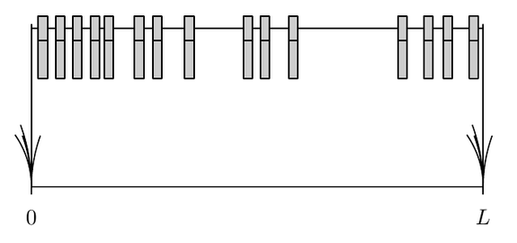
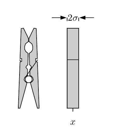
We consider the problem of hard "spheres" in one dimension, so-called "clothe pins". We are interested in sampling configurations from the microcanonical equilibrium distribution, where all allowed configurations have the same probability. The pins are attached on a line of length $L$, and have a width equal to $2\sigma$. A configuration is allowed when pins do not overlap and lie on the segment $[0,L]$.
Naive sampling for N clothes-pins
Here is the naive pin-sampling algorithm. It has an extremely high rejection rate, so do not really expect it to terminate in any reasonable time.
import random, pylab
%matplotlib inline

N = 15; L = 10; sigma = 0.1; statistics = 200 #00
data = []
rejected = 0
for iter in range(statistics):
    while True:
        x_sorted = sorted([random.uniform(sigma, L - sigma) for k in range(N)])
        min_dist = min(x_sorted[k + 1] - x_sorted[k] for k in range(N - 1))
        if min_dist > 2*sigma: break
        else: rejected += 1
    data += x_sorted
print "Fraction of accepted:", float(statistics)/rejected
pylab.title('Density of '+str(N)+' clothes-pins with sigma='+str(sigma)+' on a line of length L='+str(L))
pylab.hist(data,bins=100,normed=True)
pylab.savefig('clothes_pins.png')
pylab.show()

Interlude: computing the partition function
Let's consider a function $$\pi(x_0,\ldots,x_{N−1})$$ of the positions $x_i$'s of the $N$ pins characterising whether or not a configuration is allowed: $$\pi(x_0,\ldots,x_{N−1})=\begin{cases} 1 & \text{if allowed}\\ 0 & \text{if not allowed} \end{cases}$$ The partition function writes (for distinguishable pins) $$Z_{N,L}=\frac1{N!}\idotsint\limits_{[σ,L−σ]^N}d^Nx \;\pi(x_0,\ldots,x_{N−1})$$ Explain why $$Z_{N,L}=\idotsint\limits_{[σ,L−σ]^N}d^Nx \;\pi(x_0,\ldots,x_{N−1})\Theta(x_0<\cdots < x_{N−1})$$ where $\Theta(x_0< \cdots< x_{N−1})$ is a characteristic function, equal to 1 if $x_0 < \cdots < x_{N−1}$ and equal to otherwise.
Show that $$ Z_{N,L}=\begin{cases} (L−2N\sigma)^N/N!& \text{if }L>2N\sigma \\ 0 & \text{otherwise} \end{cases} $$
Rejection-free sampling algorithm
We thus see that the effective space in which all positions live is the segment $[0,L-2N\sigma]$. To sample a configuration, one may thus sample $N$ reals $y_i$ (with $i$ running from 0 to $N-1$) in this segment, sort them, and define the positions of the pins by adding $(2i+1)\sigma$ to the $i$th of them.
Direct_pin: rejection-free sampling of the clothes-pin configurations -- standard loops
The below programs implement the direct-sampling without rejections for the clothes-pins. It directly generates the histogram of the particle positions.
N = 11; L = 20; sigma = 0.7; statistics = 50000
data = []
for stat in range(statistics):
    y_unsorted = []
    for i in range(N):
        y_unsorted.append(random.uniform(0, L - 2*N*sigma))
    y_sorted = sorted(y_unsorted)
    x = []
    for i in range(N):
        x.append(y_sorted[i] + (2*i+1)*sigma)
        data.append(x[i])

pylab.title('Density of '+str(N)+' clothes-pins with sigma='+str(sigma)+' on a line of length L='+str(L))
pylab.hist(data,bins=500,normed=True)
pylab.show()

Direct_pin: rejection-free sampling of the clothes-pin configurations -- using list comprehension
Here is a condensed version of the above program using list comprehensions.
N = 17; L = 20; sigma = 0.5; statistics = 500000

data = []
for stat in range(statistics):
    y_sorted = sorted([random.uniform(0, L - 2 * N * sigma) for k in range(N)])
    data += [(y_sorted[k] + (2 * k + 1) * sigma) for k in range(N)]
pylab.title('Density of '+str(N)+' clothes-pins with sigma='+str(sigma)+' on a line of length L='+str(L))
pylab.hist(data,bins=1000,normed=True)

if True:
    from scipy.special import binom
    def Z(N_,L_):
        tmp = L_-2.0*sigma*N_
        if tmp>0.0: return (tmp)**N_
        else: return 0.0
    def proba(x):
        tmp = Z(N,L)
        return sum([ binom(N-1,k)*Z(k,x-sigma)*Z(N-1-k,L-x-sigma)/tmp for k in range(N) ])
    eps=1e-8
    x = pylab.linspace(sigma+eps,L-sigma-eps,1000)
    y = [ proba(x_) for x_ in x ]
    y0 = [ 1./(L-2*sigma) for x_ in x ]
    pylab.plot(x,y,'r-',x,y0,'b--')

pylab.savefig('clothes_pins.png')
pylab.show()

Density of clothes-pin centers
- The density of clothes-pin centers presents oscillations. Comment on them.
- Is this compatible with having a uniform distribution? Determine analytically the histogram for $N=2$.
- Propose an algorithm implementing periodic boundary conditions. Do you expect oscillations in this case?
- Can you extend this algorithm to more than one dimension?
from scipy.special import binom
N=5; L=10; sigma=0.7

def Z(N_,L_):
    tmp = L_-2.0*sigma*N_
    if tmp>0.0: return (tmp)**N_
    else: return 0.0
def proba(x):
    tmp = Z(N,L)
    return sum([ binom(N-1,k)*Z(k,x-sigma)*Z(N-1-k,L-x-sigma)/tmp for k in range(N) ])

eps=1e-8
x = pylab.linspace(sigma+eps,L-sigma-eps,1000)
y = [ proba(x_) for x_ in x ]
y0 = [ 1./(L-2*sigma) for x_ in x ]
pylab.plot(x,y,'r-',x,y0,'b--')
pylab.show()

Program for periodic boundary
One can add a fixed random real number between 0 and $L$ (denoted shift below) to the positions found using the rejection-free algorithm above.
statistics = 500000
data = []
for stat in range(statistics):
    y_sorted = sorted([random.uniform(0, L - 2 * N * sigma) for k in range(N)])
    shift = random.uniform(0, L)
    data += [( shift+y_sorted[k] + (2*k+1)*sigma ) % L for k in range(N)]
pylab.title('Density of '+str(N)+' clothes-pins with sigma='+str(sigma)+' on a line of length L='+str(L))
pylab.hist(data,bins=1000,normed=True)
x = pylab.linspace(0.0,L,2)
y0 = [ 1./float(L) for x_ in x ]
pylab.plot(x,y0,'b--')
pylab.savefig('clothes_pins.png')
pylab.show()

Qualitative ideas on entropic force at play in hard-core systems