Tutorial 9: Random sequential deposition 
Introduction
During the first lectures, we have seen how in Monte-Carlo algorithms one defines a dynamics (through transition probabilities) which enables to sample a given distribution $\pi(C)$ on a set of configuration $\{C\}$.
One may consider a reversed point of view, where now (e.g. physically motivated) transition rates are given, and one is interested in finding/characterizing the unknown steady state distribution. In this exercice, we focus on the problem of random sequential deposition, defined for hard disks on a one-dimensional segment (see Class Session 02).
Model
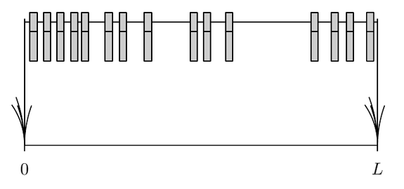
We consider the problem of hard "spheres" in one dimension, that we will call clothe pins, on a segment of length $L$. Pins of width $2\sigma$ are permanently deposited at random positions in the box provided they do not overlap with pins placed earlier. The deposition consists in trying to deposit a new pin with its center uniformly distributed in the interval $[\sigma,L–\sigma]$. This process goes on until no pins can be deposited anymore.
Time $t$ is defined as follows: the first deposition takes place at $t = 1$, and $t$ is increased by 1 at each (successfull or not) tentative deposition. One is interested for instance in the last deposition time, and in the statistical properties of the final configuration. One could also study the density as a function of time, and the dynamical approach towards the fully packed state.
- Is this problem equivalent to the one-dimensional hard sphere problem of Class Session 02? Why (Why not)?
Naive algorithm
The following (naive) algorithm implements the sequential deposition up to time $t_{\text{max}}$:
import math,random,pylab
%matplotlib inline

random.seed(3456789732)
N = 1; L = 10; sigma = 0.1; tmax = 80;
def dist(a,b): return math.fabs(b - a)
def allowed(positions,newpos):
    dists=[ dist(pos,newpos) for pos in positions ]
    return min(dists) > 2*sigma
positions=[ random.uniform(sigma,L-sigma) ]
lastt = 1
for t in range(tmax):
    pos = random.uniform(sigma,L-sigma);
    if allowed(positions,pos):
        positions.append(pos)
        lastt = t
        N += 1
        print 'pin number ',N, ',  deposition time: ',t
print '\n last deposition time: ',lastt, ' < tmax =',tmax
height = .33 * L
square = pylab.Rectangle((sigma,0), L-2*sigma, height,  fc='b')
pylab.gca().add_patch(square)
for x in positions:
    whiterec = pylab.Rectangle((x-2*sigma,0), 4*sigma,height, fc='w',ec='w')
    pylab.gca().add_patch(whiterec)
for x in positions:
    redrec = pylab.Rectangle((x-sigma,0), 2*sigma,height,  fc='r')
    pylab.gca().add_patch(redrec)
pylab.axis('scaled')
pylab.axis([0,L,0,height])
pylab.title('Clothe pins are in red, remaining available space for is in blue.')
pylab.show()

In this algorithm:
- Is the rejection probability increasing with time?
- Do you know when to stop the deposition?
Faster-than-the-clock algorithm
The idea
Consider a given configuration of the system.
- Write the rejection probability $\lambda$ in terms of the accessible length and of the total deposition length.
- Starting from a given configuration, we define taccept as the number of time steps one has to wait before the deposition of a new pin (occurring in $t_{\text{accept}}+1)$ is accepted. Determine the probability distribution of taccept.
- How would you sample this probability?
Implementation of the faster than the clock algorithm
import math,random,pylab
%matplotlib inline

#random.seed(34567897)
N = 1; L = 1000.; sigma = 0.5;
intervals = [(sigma,L-sigma)]   # list of the (ak,bk)
dists = [b-a for (a,b) in intervals]
positions = []
time = 0

def tower(data,Upsilon):
    sums = [0]
    for d in data: sums.append(d+sums[-1])
    sums.pop(0)
    for k in range(len(sums)):
        if Upsilon < sums[k]:
            break
    return k

times = []
while len(intervals) > 0:
    length = sum(dists)
    # choice of the time jump
    lambd = 1 - length/(L-2*sigma); # rejection rate
    deltat = 1
    if (lambd > 0.):
        deltat += int(math.log(random.random())/math.log(lambd))
    time += deltat
    N += 1
    times.append(time/L)
    # evolution
    Upsilon = random.uniform(0,length)
    k = tower(dists,Upsilon)
    d2 = sum(dists[p] for p in range(k+1))-Upsilon
    (a,b) = intervals.pop(k)
    dists.pop(k)
    newpos = b - d2
    positions.append(newpos)
    d1 = newpos - a;
    if (d1 > 2*sigma):
        intervals.append((a,newpos-2*sigma));dists.append(newpos-2*sigma-a)
    if (d2 > 2*sigma):
        intervals.append((newpos+2*sigma,b));dists.append(b-newpos-2*sigma)

print 'total pin number: ',N,' ultimate deposition time: ',time
print 'final time density:', 2*sigma*N/float(L)
Comparison with analytical result
This problem can actually be solved exactly (Renyi 1958) and yields the following time-evolution for the density: $$ \rho(t) = \int_0^t du\;\exp\left\{-2\int_{0}^u\frac{dv}{v}(1-e^{-v})\right\} $$ The infinite time limit turns out to be $\rho^{\infty}=0.747597920253\ldots\simeq 75\%$ which is significantly lower than the optimal packing of one.
import numpy as np
from matplotlib import rc
rc('font',**{'family':'sans-serif','sans-serif':['Helvetica']})
rc('text', usetex=True)
from scipy.integrate import quad
F = lambda u: quad(lambda x: (1.-math.exp(-x))/x, 0.0,u)[0]
analytic = lambda t: quad(lambda x: math.exp(-2.*F(x)), 0.0,t)[0]
print 'Analytical result: ', analytic(np.inf)
ts = np.logspace(-3,3,50)
pylab.semilogx(ts,map(analytic,ts))
pylab.semilogx(times,2*sigma*np.arange(1,N)/float(L),'+r')
pylab.ylabel("$\\rho(t)$",size=24)
pylab.xlabel('$t/L$',size=24)
pylab.show()

height = .33*L
square = pylab.Rectangle((sigma,0), L-2*sigma, height,  fc='b')
pylab.gca().add_patch(square)
for x in positions:
    whiterec=pylab.Rectangle((x-2*sigma,0), 4*sigma,height, fc='w',ec='w')
    pylab.gca().add_patch(whiterec)
for x in positions:
    redrec=pylab.Rectangle((x-sigma,0), 2*sigma,height,  fc='r')
    pylab.gca().add_patch(redrec)
pylab.axis('scaled')
pylab.axis([0,L,0,height])
pylab.show()
References
- Y. Pomeau, Some asymptotic estimates in the random parking problem, J. Phys. A: Math. Gen. 13 L193 (1980)
- V. Privman, J.-S. Wang, and P. Nielaba, Continuum limit in random sequential adsorption, Phys. Rev. B 43 3366 (1991)