Exact diagonalization : lecture 2
Using symmetries in the Heisenberg model
Using symmetries in the Heisenberg model
Goals : gain using symmetries
- we can list energies by quantum numbers : magnetization, dispersion relations
- we can lift degeneracies due to symmetries
- there is first a significant gain in Hilbert space dimension : consider a chain in the $S_{tot}^z =0 $ sector
from scipy.special import binom
def withcomas(i): return "{:,}".format(int(i))

L = 32
print("Ising hilbert space dimension :", withcomas(2**L))
print("with Sz conservation :", withcomas(binom(L,L//2)))
print("with Sz conservation and translations :", withcomas(binom(L,L//2)/L) )
print("with Sz conservation and translations and parity and spin inversion :", withcomas(binom(L,L//2)/(4*L)) )
Examples uses python 3 and calculations will be done on the blackboard
Conservation of total spin
Good quantum numbers
We consider spin one-half from now on. For the Heisenberg and XXZ model, the total spin $S^z_{tot} = \sum\limits_{j=1}^L S^z_j$ along $z$ is a conserved quantity. The Hamiltonian does not change the number of up and down spins. If you see up spins as particles, it is equivalent to say that the number of particles is conserved. This is associated to the $U(1)$ symmetry rotation around $z$. For an Heisenberg model, the Hamiltonian is invariant under rotation in spin space which makes it commutes with the total spin operator $\vec{S}_{tot}$. This rotation symmetry is an $SU(2)$ symmetry and we can a priori also use the quantum number ${S}_{tot}$ associated to the eigenvalues ${S}_{tot}({S}_{tot}+1)$ of the operator $\vec{S}_{tot}^2$. Actually, in the standard basis of spin up and down, $\vec{S}_{tot}^2$ is not diagonal $$ \vec{S}_{tot}^2 = L\frac 34 + 2\sum_{i<j}\vec{S}_i\cdot\vec{S}_j $$ so that it will not be straightforward to use it. Yet, there will be degeneracies between some $S^z_{tot}$ sectors correponding to the same $\vec{S}_{tot}$.
In practice, we will use $\vec{S}^z_{tot}$ only to reduce the Hilbert space dimension and the value of $\vec{S}_{tot}$ may be infered by degeneracies or applying $\vec{S}_{tot}^2$ to an eigenstate. The possible values of $S^z_{tot}$ are $- L/2, -L/2+1,\ldots,-1,0,1,\ldots,L/2-1,L/2$ for $L$ even and $- L/2, -L/2+1,\ldots,-1/2,1/2,\ldots,L/2-1,L/2$ for $L$ odd.
Naive filtering of configurations
The library is the same as before, just update Hilbert space construction. Lots of rejections.
class Conf(object):
    "A namespace for functions on configurations"

    def bitcount(c,L):
        "counts number of 1 in binary representation of a conf integer"
        return np.binary_repr(c,L).count("1")

class HeisenbergHilbert(object):
    "Hilbert space for the Heisenberg model"

    def __init__(self, L=1, Sz=0, build=True):
        "description is a list containing the local hilbert space at site i"
        self.L = L
        self.Sz = Sz
        self.ups = int((L+2*Sz)/2)
        self.hilbertsize = int(binomial(self.L,self.ups))
        if build: self.create()

    def createNaive(self):
        self.Confs = {}
        ind = -1
        for conf in range(2**self.L):
            if Conf.bitcount(conf,self.L) == self.ups:
                ind += 1
                self.Confs[conf] = ind
        if not self.hilbertsize == len(self.Confs):
            print("Error in hilbert dimension")
from heisenberg import *

print(HeisenbergHilbert(L=4,Sz=0))
print(HeisenbergHilbert(L=3,Sz=1/2))
print(HeisenbergHilbert(L=7,Sz=-3/2))
Using tensorial product
Implementation using tensorial product of configurations. System is split into two halves with left and right configurations : $|\text{conf}\rangle = |L\rangle\otimes|R\rangle$. We use $$ S_{tot}^z = S_L^z + S_R^z $$ Much less rejections. Yet, not optimal, there exist algorithms without rejection but this one is easily generalizable to other additive quantum numbers and has a transparent physical intepretation.
class HeisenbergHilbert(object):
    "Hilbert space for the Heisenberg model"

    def create(self):
        def SortByQn(Ls,kmin,kmax):
            res = {}
            for conf in range(2**kmin-1,((2**kmax-1)<<(Ls-kmax))+1):
                k = Conf.bitcount(conf,Ls)
                if kmin <= k <= kmax:
                    if not k in res: res[k] = [conf]
                    else: res[k].append(conf)
            return res
        if self.L <= 2:
            self.createNaive()
            return
        LL = self.L-self.L//2
        LR = self.L//2
        leftConfs  = SortByQn(LL,max(0,self.ups-LR),min(self.ups,LL))
        rightConfs = SortByQn(LR,max(0,self.ups-LL),min(self.ups,LR))
        self.Confs = {}
        ind = -1
        halfshift = self.L//2
        for kl in leftConfs.keys():
            for lconf in leftConfs[kl]:
                kr = self.ups - kl
                if kr in rightConfs.keys():
                    for rconf in rightConfs[kr]:
                        ind += 1
                        self.Confs[(lconf<<halfshift)^rconf] = ind
        if not self.hilbertsize == len(self.Confs):
            print("Error in hilbert dimension")
from heisenberg import *

L=26
print("Bare Ising dimension :",withcomas(2**26))
print(HeisenbergHilbert(L=L,Sz=0))
Off-diagonal operators
Some operators may change the total spin of the system. It will take configurations from a subspace as input and outputs configurations in another one.
class OffDiagOperator(object):

    def __init__(self,hilbert):
        "Hilbert is the target hilbert space"
        self.hilbert = hilbert

    def __mul__(self,psi):
        res = zeroWf(self.hilbert)
        for conf, i in psi.hilbert.Confs.items():
            coef, newconf = self.Apply(conf)
            if newconf != conf:
                j = self.hilbert.Confs[newconf]
                res[j] += coef * psi[i]
        return res

    def __str__(self):
        return self.name


class Sp(OffDiagOperator):
    def __init__(self,hilbert,site):
        OffDiagOperator.__init__(self,hilbert)
        self.site = site
        self.name = "Sp_"+str(site)
    def Apply(self,conf):
        return 1, conf|(1<<self.site)
from heisenberg import *

hstart = HeisenbergHilbert(L=4,Sz=0)
hend = HeisenbergHilbert(L=4,Sz=1)

psi1 = randomWf(hstart)
psi2 = Sp(hend,2)*psi1
print(psi1.readable())
print(psi2.readable())
Translation symmetry
Translation invariance
We want to use translational invariance in the case where the Hamiltonian is invariant under translation. For single-particle, the usual framework is Bloch theorem.
On a lattice, we'll use a discrete version of the analysis. Consider a chain of length $L$ with periodic boundary conditions. Let $T$ be the translation of one site to the right. An example of its action is $$ T|{\uparrow\downarrow\uparrow\downarrow\uparrow}\rangle = |{\uparrow\uparrow\downarrow\uparrow\downarrow}\rangle $$ Let's write $|k\rangle$ the eigenvectors of $T$. Since $T^L=1$, its eigenvalues are $e^{ik}$ with the momentum $k$ that satisfies $$ T |k\rangle = e^{ik} |k\rangle \quad \text{ with } k = \frac{2\pi}{L} n \quad n = 0,1,\ldots,L-1 $$ The $k$ are good quantum numbers labeling the total momentum of the states.
The translation operators corresponding to translations of $r=0,1,\ldots,L-1$ sites a simply $T_r = T^r$ and have eigenvalues $e^{ikr}$. A way to construct the eigenstates of $T$ is to introduce a symmetric invariant superposition given a starting configuration state $|a\rangle$ : given $k$, we write $$ |a(k)\rangle = \frac{1}{\sqrt{N_a}} \sum_{r=0}^{L-1} e^{-ikr}T^r |a\rangle $$ so that one can check that $T |a(k)\rangle = e^{ik} |a(k)\rangle$. The $ |a(k)\rangle $ are Bloch-states.
Some remarks :
The normalization prefactor $\frac{1}{\sqrt{N_a}}$ depends on the state and is not always $\frac{1}{\sqrt{L}}$ as in Fourier transform for the following reason : under applying $T^r$ to a state which has some periodicity, one may generate the same state again. For example, consider the Néel state with $L$ even : $$ T|{\uparrow\downarrow\uparrow\downarrow\uparrow\downarrow}\rangle = |{\downarrow\uparrow\downarrow\uparrow\downarrow\uparrow}\rangle \quad T^2|{\uparrow\downarrow\uparrow\downarrow\uparrow\downarrow}\rangle = |{\uparrow\downarrow\uparrow\downarrow\uparrow\downarrow}\rangle $$ If all $T^r |a\rangle$ are different (more common case for large systems), then the prefactor is $\frac{1}{\sqrt{L}}$.
The norm of the state can be zero depending on the quantum number. For example, considering a ferromagnetic state $|{\uparrow\uparrow\uparrow\uparrow\uparrow\uparrow}\rangle$ which will always be invariant under translation, if $k=\pi$, the alternating $e^{-ikr}=\pm 1$ builds a null state.
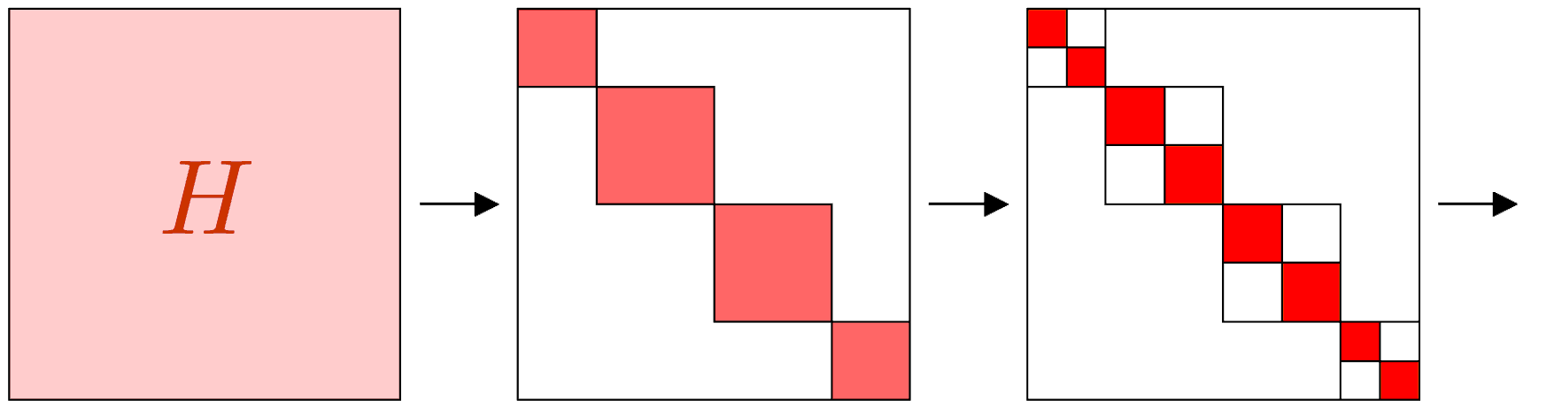
One aim about using symmetries with exact diagonalization is to reduce the Hilbert space basis. It would be easy to write down the operator corresponding to the basis change to the $\{ |a(k)\rangle \}$. In this basis, the Hamiltonian would be block diagonal. Yet, the basis change matrix would involve all the non-symmetrized Hilbert space and we would not gain memory at this stage, we'll only find smaller matrices to diagonalize in each block.
The representative basis strategy
There is actually a way to directly write the block diagonal matrices without explicitly write down the basis change matrix.
Orbits and representatives
Starting from a given configuration $|a\rangle$, the states $|a(r)\rangle = T^r |a\rangle$ generated by the translation operator form a close orbit : they can all be reached from any of a given $|a(r)\rangle$ by applying $T$. The number of these states depends on the periodicity of $|a\rangle$, it is at most $L$. The total number of orbits is approximately the dimension of the non-symmetrized Hilbert space over $L$.
As any state of the orbit can be reached from only one, the idea is to keep only one per orbit. The chosen state is called the representative and is a usual configuration state $|a\rangle$, not a superposition. The choice is arbitrary and an easy numerical choice is to choose the $|a\rangle$ which bits configuration corresponds to the smallest integer.
implementation of translational symmetry
from heisenberg import *

def translate_right(conf,L):
    "translation of one site to the right"
    bs = bin(conf)[2:].zfill(L)
    return int(bs[1:]+bs[0],2)

def translate(conf,L):
    "translation of one site to the left"
    first = Conf.readsite(conf,0)
    return (conf>>1)|(first<<(L-1))

L=3
for conf in range(2**L):
    print(Conf.binconf(conf,L), Conf.binconf(translate_right(conf,L),L), Conf.binconf(translate(conf,L),L))
Selection of the representatives : norm and periodicity
The periodicity $R_a$ of a representative $|a\rangle$ is defined as the smallest integer such that $T^{R_a} |a\rangle = |a\rangle$. $R_a$ may take the values $1,2,\ldots,L$. Taking this periodicity into account, one can write the Bloch-state in the following way: $$ |a(k)\rangle = \frac{F(k,R_a)}{\sqrt{N_a}} \sum_{u=0}^{R_a-1} e^{-iku}T^u |a\rangle $$ with $$ F(k,R_a) = \sum_{n=0}^{L/R_a-1} e^{-ikR_a n} = \begin{cases} L/R_a & \text{ if } kR_a = 0 \;[2\pi] \\ 0 & \text{otherwise} \end{cases} $$ When trying to find $N_a$ that normalizes $|a(k)\rangle$, one finds $N_a = R_a|F(k,R_a)|^2$. When $F(k,R_a)=0$, the representative is not allowed in this symmetry sector (given $k$) and must be excluded. If allowed, the normalization factor then reads $$ N_a = \frac{L^2}{R_a} $$ and, since $kR_a$ is a multiple of $2\pi$, we can write $$ k = \frac{2\pi}{R_a}m\qquad m=0,1,\ldots,R_a-1 $$
implementation of the basis construction and the inverse search basis
class HeisenbergHilbert(object):
    "Hilbert space for the Heisenberg model"

    def __init__(self, L=1, Sz=0, k=0, build=True):
        "description is a list containing the local hilbert space at site i"
        self.L = L
        self.Sz = Sz # total spin sector
        self.k = k   # integer number between 0 and L-1 momentum=2*pi/L*k
        self.ups = int((L+2*Sz)/2)
        self.hilbertsize = int(binomial(self.L,self.ups))
        self.nconf = -1  # counter
        self.basis = []  # to store couples (|a>,R_a)
        self.invbasis = {} # to get index of |b> and corresponding R_b
        if build: self.create()

    def index(self,conf):
        "returns the index of a configuration"
        return self.invbasis[conf][0]

    def checkstate(self,conf):
        t = conf
        for r in range(self.L):
            t = Conf.translate(t,self.L)
            if t < conf:
                return -1
            elif (t == conf):
                if (np.mod(self.k,self.L/(r+1)) != 0):
                    return -1
                else:
                    return r+1

    def fillhilbert(self,conf):
        R = self.checkstate(conf)
        if R >0:
            self.nconf +=1
            self.basis.append( (conf,R) )
            self.invbasis[conf] = (self.nconf,R)

    def create(self):
        def SortByQn(Ls):
            res = {}
            for conf in range(2**Ls):
                k = Conf.bitcount(conf,Ls)
                if not k in res: res[k] = [conf]
                else: res[k].append(conf)
            return res
        if self.L <= 2:
            self.createNaive()
            return
        leftConfs  = SortByQn(self.L-self.L//2)
        rightConfs = SortByQn(self.L//2)
        halfshift = self.L//2
        for kl in leftConfs.keys():
            for lconf in leftConfs[kl]:
                kr = self.ups - kl
                if kr in rightConfs.keys():
                    for rconf in rightConfs[kr]:
                        conf = (lconf<<halfshift)^rconf
#---------------- new part ------------------------------
                        self.fillhilbert(conf)
#--------------------------------------------------------
        self.hilbertsize = len(self.basis)
Matrix elements
We assume that the Hamiltonian commutes with $T$ and that it can be decomposed into $H = \sum_{\alpha} h_{\alpha}$ of elementary operators that are called non-branching operators : given a configuration, $h_{\alpha}$ will generate only one other configuration but not a superposition.
Consider a given representative $|a\rangle$. Applying $h_{\alpha}$ gives $h_{\alpha}|a\rangle = h_{\alpha}(a)|b'_{\alpha}\rangle$ in which $h_{\alpha}(a)$ is the coefficient associated to the action of the operator (the same as if there were no symmetries) and $|b'_{\alpha}\rangle$ the new configuration (which depends and is close to $|a\rangle$ but we only keep the dependence on $\alpha$ in the notation).
$|b'_{\alpha}\rangle$ is not necessarily a representative. Let us call $|b_{\alpha}\rangle$ the corresponding representative of $|b'_{\alpha}\rangle$. In the orbit, the are connected by $T$ so there exists an integer $\ell_{\alpha}$ such that $|b'_{\alpha}\rangle = T^{-\ell_{\alpha}}|b_{\alpha}\rangle$.
With this, one can show that the matrix elements of the symmetrized hamiltonian can be computed directly and only from the knowledge of the representatives and from the determination of $\ell_{\alpha}$ and the $R_a$. Indeed : for two representatives $|a\rangle$ and $|b\rangle$, the matrix elements between their associated Bloch-states reads $$ \langle{b(k)}|{H}|{a(k)}\rangle = \sum_{\alpha\text{ connecting } a\to b} h_{\alpha}(a)e^{-ik\ell_{\alpha}}\sqrt{\frac{R_a}{R_b}} $$ Important : such formula works any operator that commutes with $T$ (not only the Hamiltonian), one has for keep this in mind when measuring observables. Then, one has to use symmetrized version of the observable you want. Let $O_j$ be a local observable, then the symmetrized version will be $$ O = \frac 1 L \sum_{j=0}^{L-1} O_j $$
class HeisenbergHilbert(object):
    "Hilbert space for the Heisenberg model"

    def representative(self,conf):
        rep = conf; t = conf; l = 0
        for r in range(self.L):
            t = Conf.translate(t,self.L)
            if (t < rep):
                rep = t; l = r+1
        return rep, l

class Operator:

    def __mul__(self,psi):
        res = zeroWf(psi.hilbert,dtype=psi.dtype)
        for i in range(psi.hilbert.hilbertsize):
            conf,Ra = psi.hilbert.basis[i]
            coef, newconf = self.Apply(conf)
            if newconf != conf:
                repb, l = psi.hilbert.representative(newconf)
                if repb in psi.hilbert.invbasis.keys():
                    j, Rb = psi.hilbert.invbasis[repb]
                    k = 2*np.pi*psi.hilbert.k/psi.hilbert.L
                    res[j] += coef * np.exp(-1j*k*l)*np.sqrt(Ra/Rb) * psi[i]
            else:
                res[i] += coef * psi[i]
        return res
from heisenberg import *
np.set_printoptions(precision=9,suppress=True)

def HeisenbergHam(L):
    HamZZ = GeneralOp([ [ 1.0, SzSz(i,(i+1)%L)] for i in range(L) ])
    HamXY = GeneralOp([ [ 1.0, Spinflip(i,(i+1)%L)] for i in range(L) ])
    return HamZZ + HamXY

L=8
hilbert = HeisenbergHilbert(L=L,Sz=0)
Ham = HeisenbergHam(L)
print(Ham.Energies(hilbert,num=hilbert.hilbertsize,algorithm="Fulldiag")[:40])
from heisenberg_trans import *

def HeisenbergHam(L):
    HamZZ = GeneralOp([ [ 1.0, SzSz(i,(i+1)%L)] for i in range(L) ])
    HamXY = GeneralOp([ [ 1.0, Spinflip(i,(i+1)%L)] for i in range(L) ])
    return HamZZ + HamXY

def fullspectrum(L=2,Sz=0):
    E = np.array([])
    for k in range(L):
        hilbert = HeisenbergHilbert(L=L,Sz=Sz,k=k)
        Ham = HeisenbergHam(L)
        if hilbert.hilbertsize>0:
            E = np.append(E,Ham.Energies(hilbert,num=hilbert.hilbertsize,algorithm="Fulldiag"))
    return np.sort(E)

np.set_printoptions(precision=9,suppress=True)
print(fullspectrum(L=8,Sz=0)[:40])
Downloading the module
python 3
- http://lptms.u-psud.fr/membres/groux/Test/ED/heisenberg.py
- http://lptms.u-psud.fr/membres/groux/Test/ED/heisenberg_trans.py
python 2
References
- Anders Sandvik lectures notes at : http://physics.bu.edu/~sandvik/vietri/index.html The translational symmetry presentation is very close to these lecture notes.