Exact diagonalization : tutorial 2
Heisenberg spin chains
Heisenberg spin chains
Dispersion relations
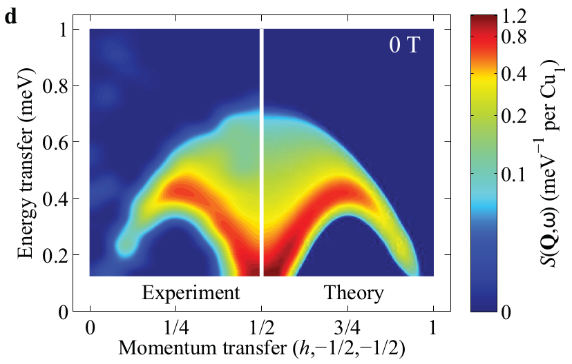
Dispersion relations are the energy of elementary excitations above the ground-state of energy $E_0$ : $$ \omega(k) = E(k)-E_0 \;. $$ They can be typically probed by neutron scattering experiments on quantum magnets materials : here is an example of comparison between experiment and Bethe-ansatz based numerical calculations on the antiferromagnetic Heisenberg chain.
Non-frustrated chains
Ferromagnetic chain : deviation states
1/ What is the ground-state(s) of the ferromagnetic Heisenberg chain on length $L$ ? What is its energy and total spin ?
2/ An elementary excitation above the ground-state is obtained by flipping a spin at site $j$. This state will be denoted by $|{j}\rangle$. What is the total spin of this state ? Apply the Hamiltonian and show that the Hamtiltonian has a simple form in the $\{|{j}\rangle\}$ basis
3/ By introducing the Fourier transform $$ |{k}\rangle = \frac{1}{\sqrt{L}} \sum_{j=0}^{L-1} e^{ikj} |{j}\rangle $$ find the energies $\varepsilon(k)$ of the single-deviation states. Infer that the dispersion relation $\omega(k)$ of the single-deviation states for the ferromagnetic chain ($J<0$) reads $$ \omega_1(k) = -J(1-\cos(k)) $$
4/ For two deviations states, explains qualitatively why there is a continuum between $$ \omega_2(k) = -2J(1\pm \cos(k/2)) $$ and a bound state, the dispersion of which is given as $$ \omega_2^b(k) = -J/2(1-\cos(k)) . $$ Look at the $k \to 0$ limit of single-deviation states and obtain an effective mass for a single deviation. Justify the prefactor $J/2$ of the bound state ?
5/ Observe what happens when the number of deviations increases by setting maxdev = 3 and interpret the lowest-energy states. What happens in the thermodynamical limit ? How can the SU(2) symmetry be broken ?
from heisenberg_trans import *

def HeisHam(L=4):
    Ham = GeneralOp([ [ -1.0, SzSz(i,(i+1)%L)] for i in range(L) ])
    Ham+= GeneralOp([ [ -1.0, Spinflip(i,(i+1)%L)] for i in range(L) ])
    return Ham

def dispersion(L,sz=0,algo="Arnoldi"):
    Ek = {}
    for k in range(L//2+1):
        hilbert = HeisenbergHilbert(L=L,Sz=sz,k=k)
        Ham = HeisHam(L=L)
        E = Ham.Energies(hilbert,num=100,algorithm=algo)
        Ek[k] = E[:]
    E0 = -1/4*L # the energy of the ferromagnetic ground-state
    for k in Ek.keys():
        Ek[k] -= E0
    return Ek

from pylab import *
%matplotlib inline

L=20
colors = { 1:'r', 2:'b', 3:'g', 4:'y' }
maxdev = 4
for dev in range(maxdev,0,-1):
    Ek = dispersion(L,sz=L/2-dev,algo="Fulldiag")
    for k in Ek.keys():
        Ks = 2*np.pi*k/L*np.ones(len(Ek[k]))
        scatter(Ks,Ek[k],color=colors[dev])
# exact results
k = np.linspace(0,np.pi,101)
exact_single = lambda k : 1-np.cos(k)
plot(k,exact_single(k),'r-')
exact_two_up = lambda k : 2*(1+np.cos(k/2))
plot(k,exact_two_up(k),'b-')
exact_two_dn = lambda k : 2*(1-np.cos(k/2))
plot(k,exact_two_dn(k),'b-')
exact_two_b = lambda k : 0.5*(1-np.cos(k))
plot(k,exact_two_b(k),'b-')
xlabel("$k$",fontsize=20)
ylabel("$\omega(k)$",fontsize=20)
xlim(0-0.1,np.pi+0.1)
ylim(0,4.0)
tight_layout()
show()

Antiferromagnetic chain : spin-wave theory and Bethe-ansatz results
The exact dispersion relation for the antiferromagnetic chain reads $$ \omega(k) = \frac{\pi}{2}J \sin(k) $$
6/ Take the $k \to 0$ limit. What is the nature of low-energy excitations in this regime and their natural speed ? Why is there another branch at $k = \pi$ ?
from heisenberg_trans import *

def HeisHam(L=4):
    Ham = GeneralOp([ [ 1.0, SzSz(i,(i+1)%L)] for i in range(L) ])
    Ham+= GeneralOp([ [ 1.0, Spinflip(i,(i+1)%L)] for i in range(L) ])
    return Ham

def dispersion(L,num=1,algo="Arnoldi"):
    Ek = {}
    for k in range(L//2+1):
        hilbert = HeisenbergHilbert(L=L,Sz=0,k=k)
        Ham = HeisHam(L=L)
        E = Ham.Energies(hilbert,num=num,algorithm=algo)
        Ek[k] = E[:]
    E0 = min(e[0] for e in Ek.values())
    for k in Ek.keys():
        Ek[k] -= E0
    return Ek

from pylab import *
%matplotlib inline

for L in [10,12,14,16,18,20]:
    Ek = dispersion(L,num=4)
    for k in Ek.keys():
        Ks = 2*np.pi*k/L*np.ones(len(Ek[k]))
        scatter(Ks,Ek[k])
k = np.linspace(0,np.pi,101)
exact = lambda k : np.pi/2*np.sin(k)
plot(k,exact(k),'r-')
xlabel("$k$",fontsize=20)
ylabel("$\omega(k)$",fontsize=20)
xlim(0-0.1,np.pi+0.1)
ylim(0,2.0)
tight_layout()
show()

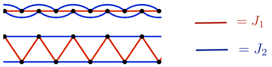
The Majumdar-Ghosh point $J_2=J_1/2$
No questions, only qualitative discussion. Analytical calculations to derive the MG state.
A good approximation of the exact dispersion relation reads, for the singlet excitation : $$ \omega(k) = J_2\left[ \frac 5 2 + 2\cos(k)\,\text{sign}(k-\pi/2) \right] $$
from heisenberg_trans import *

def J1J2(L=4,J2=0.0):
    Ham = GeneralOp([])
    Ham+= GeneralOp([ [ 1.0, SzSz(i,(i+1)%L)] for i in range(L) ])
    Ham+= GeneralOp([ [ 1.0, Spinflip(i,(i+1)%L)] for i in range(L) ])
    if not J2==0.0:
        Ham+= GeneralOp([ [ J2, SzSz(i,(i+2)%L)] for i in range(L) ])
        Ham+= GeneralOp([ [ J2, Spinflip(i,(i+2)%L)] for i in range(L) ])
    return Ham

def dispersion(L,J2=0.0,num=1,algo="Arnoldi"):
    Ek = {}
    for k in range(L//2+1):
        hilbert = HeisenbergHilbert(L=L,Sz=0,k=k)
        Ham = J1J2(L=L,J2=J2)
        E = Ham.Energies(hilbert,num=num,algorithm=algo)
        Ek[k] = E[:]
    E0 = min(e[0] for e in Ek.values())
    for k in Ek.keys():
        Ek[k] -= E0
    return Ek

from pylab import *
%matplotlib inline

J2 = 0.5
for L in [8,12,16,20]:
    Ek = dispersion(L,J2=J2,num=4)
    for k in Ek.keys():
        Ks = 2*np.pi*k/L*np.ones(len(Ek[k]))
        scatter(Ks,Ek[k])
k = np.linspace(0,np.pi,101)
exact = lambda k : J2*(5/2+2*np.sign(k-np.pi/2)*np.cos(k))
plot(k,exact(k),'r-')
xlabel("$k$",fontsize=20)
ylabel("$\omega(k)$",fontsize=20)
xlim(0-0.1,np.pi+0.1)
ylim(0,1.6)
tight_layout()
show()
