T-II-2new

Variational methods: Sound waves in solid and fluid materials

     

Consider a solid body or a fluid at rest. Under the action of an external force it will start to move or flow and the work done the force is transformed in kinetic energy. This is the case of a rigid body or an incompressible fluids, but in real materials part of the work can be used to induce a deformation. A compression for example has an ergetic cost both for fluids and solids, while a change in shape (shear) has a cost only for solids.

If the deformation is not too large the work is stored in terms of elastic energy and it is reversibly released when the force is removed. As a consequence, after a sudden pertubation, elastic waves propagates in the material. Similarly to light, which are waves associated to the electromagnetic field, the sound that we can ear are waves associated to the elastic field. But which field?

At variance with their electromagnetic cousins, elastic waves can propagate only inside materials and display a quite different nature in solids with respect to fluids. Here we derive their equations of motion in both kind of material and compute their speed.

Part I: Elasticity in solids

     

The first succesful attempt to describe deformations in solids is provided by the theory of elasticity. The theory is based on the assumptions that (1) the solid body can modeled as a continuum medium and (2) the energetic cost of the deformation is kept at the lowest order in perturbation. The fundamental equations of elasticity have been established by Cauchy and Poisson in the twenties of the 19th century, well before the discovery of the atomic structure of matter.

     

Displacement fields and strain tensor

     

Here we review the basic objects of elastic theory that you have done last year (e.g. see pages 62-66 of Mécanique du solide et des matérieaux, partie 1, Pascal Kurowski).

Consider a perfectly isotropic continuum medium with density mass $\rho _{0}$ at equilibrium:. Assume that at time $t=0$ a body is at rest and no external forces are applied. Each point of the body can be identified with its postion in the space:

${\vec {r}}=(x_{1}=x,x_{2}=y,x_{3}=z)$

Then under the action of external forces the body starts to be deformed: the point located in ${\vec {r}}$ moves to a new location ${\vec {r}}_{\text{new}}$ at time $t>0$ . The displacement, ${\vec {u}}={\vec {r}}_{\text{new}}-{\vec {r}}$, differs from point to point of the body and is then a field, namely a function of the original position ${\vec {r}}$:

${\vec {u}}({\vec {r}},t)=\left(u_{1}({\vec {r}},t),u_{2}({\vec {r}},t),u_{3}({\vec {r}},t)\right)$

the displacement field encodes then all information about the deformation.

However large displacements does not always correspond to large deformation as the body can move rigidly without deformation. To quantify how much a body is deformed it is useful to introduce the symmetric strain tensor $\epsilon _{ik}$ :

$\epsilon _{ik}={\frac {1}{2}}\left(\partial _{k}u_{i}+\partial _{i}u_{k}\right)\,,\quad {\text{with}}\;\partial _{k}={\frac {\partial }{\partial x_{k}}}\quad (1)$

Q1: Take two points at a distance $d\ell$ and compute the distance $d\ell _{\text{new}}$ after a small deformation. Show that at the lowest order in the deformation it can be written as

$d\ell _{\text{new}}^{2}\approx d\ell ^{2}+2\sum _{i,k}\epsilon _{ik}dx_{i}dx_{k}$

Compression: the (relative) density field

     

Consider now a local compression at the point ${\vec {r}}$. The volume element around the point, $dV=dx_{1}\,dx_{2}\,dx_{3}$, is squeezed to a smaller volume $dV_{\text{new}}$ and the density mass will locally increases from the uniform value $\rho _{0}$:

$\rho ({\vec {r}},t)=\rho _{0}+\delta \rho ({\vec {r}},t)=\rho _{0}\left(1+\sigma ({\vec {r}},t)\right)$

The scalar field $\sigma ({\vec {r}},t)$ represents the relative fluctuation of the density.

$\sigma ({\vec {r}},t)={\frac {\rho ({\vec {r}},t)-\rho _{0}}{\rho _{0}}}=-{\frac {dV_{\text{new}}-dV}{dV}}$

Q2: Show that at the first order in perturbation one has

$dV_{\text{new}}\approx dV\left(1+{\text{Tr}}(\epsilon )\right)\quad$

.

Tip: it is convenient to write the element volume in the principal coordinate around the point ${\vec {r}}$. There the symmetric deformation tensor is diagonal.

Conclude that

$\sigma ({\vec {r}},t)=-{\text{div}}({\vec {u}})$

     

In general all deformation can be represented as the sum of a uniform compression (change in volume without change of shape) and a shear (change of shape without change of volume):

$\epsilon _{ik}=\left(\epsilon _{ik}-{\frac {1}{3}}\delta _{ik}{\text{Tr}}(\epsilon )\right)+{\frac {1}{3}}\delta _{ik}{\text{Tr}}(\epsilon )\quad {\text{with}}\quad \delta _{ik}={\begin{cases}0\;{\text{if}}\;i\neq k\\1\;{\text{if}}\;i=k\end{cases}}\quad (2)$

The first term is a shear as its trace is zero. The second term is a compression/rarefaction.

Energy cost of the deformation

   

A body at rest, in abscence of external force and at thermal equilibrium does not display any deformation, this means that when the strain tensor is zero for all points, the potential energy displays a minimum. As a consequence for small deformations the first terms of the expansion of the potential energy must be quadratic in the strain tensor (elastic approximation). The more general quadratic form can be written as $\int d{\vec {r}}\sum _{ijkl}\epsilon _{ij}\,C_{ijkl}\,\epsilon _{kl}$, where the tensor $C_{ijkl}$ contains all the elastic moduli. For an isotropic material the energy cost should be frame independent and we can write a simpler quadratic form that we will discuss in class:

$E_{\text{el}}=\int d{\vec {r}}\left[{\frac {K}{2}}{\text{Tr}}(\epsilon )^{2}+\mu \sum _{ik}\left(\epsilon _{ik}-{\frac {1}{3}}\delta _{ik}{\text{Tr}}(\epsilon )\right)^{2}\right]$

The first term accounts for the cost of the change in volume, the second for the change of shape. The positive constants $K,\mu$ are respectively the bulk and the shear modulus and have dimensions of a pressure. These two constants are material dependent and fully describe its elastic properties.

   

Kinetic energy

   

The kinetic energy can then be written as

$T={\frac {\rho _{0}}{2}}\int d{\vec {r}}\left({\dot {u}}_{1}^{2}({\vec {r}},t)+{\dot {u}}_{2}^{2}({\vec {r}},t)+{\dot {u}}_{3}^{2}({\vec {r}},t)\right)$

where $\rho _{0}$ is the mass density of the material at rest. Here used the fact that the mass contained in an infinitesimal volume around the point located in ${\vec {r}}$ is $\rho _{0}\,dV=\rho _{0}\,d{\vec {r}}$.

   

Equation of motion with the variational principle

   

Q3: Show that the potential elastic energy can be re-written in the following form:

$E_{\text{el}}=\int d{\vec {r}}\left[{\frac {1}{2}}\left(K-{\frac {2}{3}}\mu \right)\left(\sum _{l}\partial _{l}u_{l}\right)^{2}+{\frac {\mu }{4}}\sum _{l,m}(\partial _{l}u_{m}+\partial _{m}u_{l})^{2}\right]$

 

The associated action is given by

$S=\int dt\int d{\vec {r}}\,{\mathcal {L}}=\int dt\int d{\vec {r}}\,\left({\mathcal {T}}_{\text{kin}}-{\mathcal {E}}_{\text{el}}\right)$

where ${\mathcal {L}}$ is the Lagrangian density, ${\mathcal {T}}$ is the kinetic energy density, and ${\mathcal {E}}_{\text{el}}$ is the potential energy density

 

Q4: Write explicitly ${\mathcal {T}},{\mathcal {E}}_{\text{el}}$.

Q5: Using the variational methods show that the equation of motion for a given component $u_{i}({\vec {r}},t)$ of the displacement writes

$\rho _{0}{\ddot {u}}_{i}=\sum _{k}{\frac {d}{dx_{k}}}{\frac {d}{d(\partial _{k}u_{i})}}{\mathcal {E}}_{\text{el}}$

Q6: Show that the 3 equations of motion take the form

$\rho _{0}{\ddot {u}}_{i}=\mu \sum _{k}{\frac {\partial ^{2}u_{i}}{\partial x_{k}^{2}}}+(K+{\frac {\mu }{3}})\sum _{k}{\frac {\partial ^{2}u_{k}}{\partial x_{i}\partial x_{k}}}$

and organize them in the vectorial form:

${\ddot {\vec {u}}}=c_{t}^{2}\nabla ^{2}{\vec {u}}+(c_{l}^{2}-c_{t}^{2}){\vec {\text{grad}}}\;{\text{div}}\,({\vec {u}})$

Q7: Provide the expression of the two constants $c_{t},c_{l}$ To make progress we will consider plane waves, namely deformations that are fonction of $(x,t)$ only.

${\vec {u}}({\vec {r}},t)={\vec {u}}(x,t)$

This means that all $y,z$ derivatives are zero.

Q8: Write the explicit form of the three wave equations. They are D'Alembert equations, explain why $c_{t},c_{l}$ are called transverse mode velocity and longitudinal mode velocity.

 

It is possible to show that the result obtained for plain waves is very general: in solids elastic waves has two transverse components propagating at velocity $c_{t}$ and one longitudinal component propagating at velocity $c_{l}>c_{t}$.

Conclude that the elastic field in fluids is the displacement vectorial field.

• 

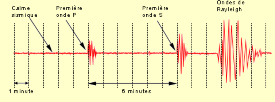
  Seismic waves recorded by a seismograph after an earthquake. Longitudinal waves are the quickest and for this reason called primary (P-waves), then arrive the transverse waves, for this reason called secondary (S-waves). Finally it's the turn of Rayleigh waves which are also solution of the D'Alembert equation but propagate only on the Earth surface. They are slower and less damped then bulk waves.

• 

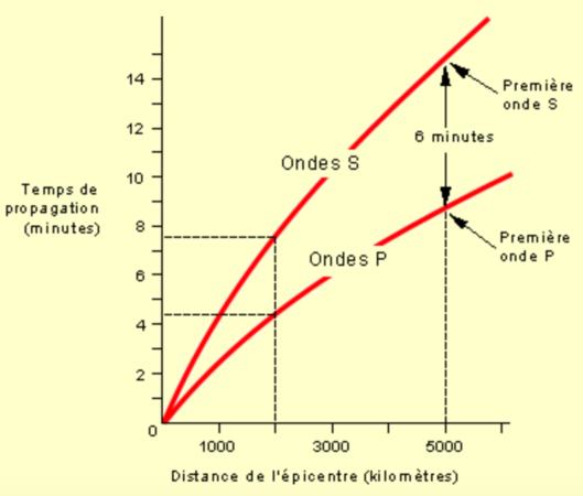
  The time delay between the P and S waves grows with seismograph-epincenter distance. The measure of three independent seismographs allows thus to identify the location of the epicenter.

Elasticity in fluids

   

A fluid does not oppose a change in its shape with any internal resistance, but displays a finite energy cost to compression. Using the same reasoning used before we can write the Lagrangian density:

${\mathcal {L}}({\vec {r}},t)={\frac {\rho _{0}}{2}}{\dot {\vec {u}}}^{2}-{\frac {K}{2}}({\text{div}}({\vec {u}}))^{2}$

Q9 Show that the associated equation of motion

$\rho _{0}\,{\ddot {\vec {u}}}=K{\vec {\text{grad}}}\left({\text{div}}({\vec {u}})\right)$

Q10 Show that the previous equation of motion corresponds to the D'Alembert Equation for the scalar field $\sigma ({\vec {r}},t)$. Conclude that the elastic field in fluids is the scalar relative density field.

• 

  Men landed on the Moon 50 years ago, but a Journey to the Center of the Earth remains science fiction. The deepest artificial holes go only 12 km into the Earth's crust.

• 

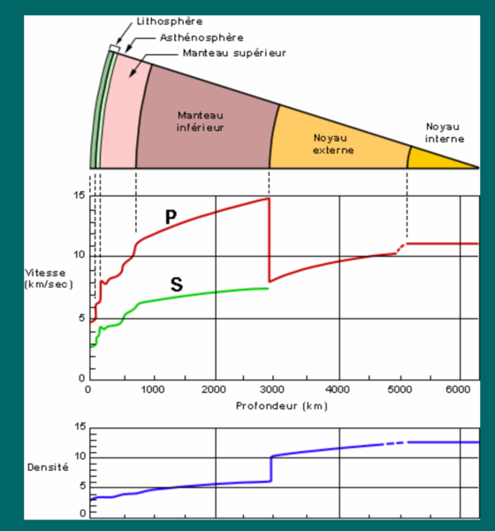
  The chemical-physical structure of the 6000 km of our planet are known by the trip reports of seismic waves. For example we know the core is fluid as secondary waves cannot travel deeper than 3000 Km.

Sound speed in perfect gas

   

Generally speaking the sound speed (the transverse one for solids) takes the form

$c_{l}={\sqrt {\frac {K+(4\mu )/3}{\rho _{0}}}}$

the constant K is much bigger in solid then liquids and much bigger in liquids then gases. For this reason sound propagates much faster in solids (6 km /s in steal) then in water (1 km /s) or, even worst, in air (331 m /s at T=273 K).

For perfect gases it is possible to evaluate the bulk modulus and then the speed sound velocity in gases. Newton did the first attempt, but he made a mistake corrected later by Laplace. Consider the gas at equilibrium at temperature $T$, pressure $P_{0}$ and density $\rho _{0}$. We consider a sudden expansion/compression from a volume $V_{0}$ around ${\vec {r}}$ to $V_{0}+\delta V$ and evaluate again the stored elastic energy. It can be written as the work associated to the expansion/compression:

$E_{\text{el}}={\frac {K}{2}}\int d{\vec {r}}{\text{Tr}}(\epsilon )^{2}={\frac {K}{2}}{\frac {(\delta V)^{2}}{V_{0}}}=-\int _{V_{0}}^{V_{0}+\delta V}\,P(V)\,dV$

the pressure can be expanded around the equlibrium

$P(V)\approx P_{0}+\left({\frac {\partial P}{\partial V}}\right)_{V=V_{0}}(V-V_{0})$

Q11: Show that

$K=-V_{0}\left({\frac {\partial P}{\partial V}}\right)_{V=V_{0}}$

   

Newton idea was that the the compressed gas remain at the same temperature $T$, so that

$PV=$ constant

Q12: Show that in this case

$K=P_{0}$

and using that at 1 atmosphere ($101325$ Pa) the density of air is $1.293$ kg/m$^{3}$ (at T=273 K)) compute the sound speed predicted by Newton.

   

However, Laplace undestood that a sound wave gas oscillates sufficiently rapidly that there is no time to thermalize. The heat is unable to flow fast enough to smooth out any temperature perturbations generated by the wave. Under these circumstances, the gas obeys the adiabatic gas law,

$PV^{\gamma }=$ constant

where $\gamma$ the ratio of specific heats (i.e., the ratio of the gas's specific heat at constant pressure to its specific heat at constant volume). This ratio is approximately $1.4$ for ordinary air.

Q13: Compute the bulk modulus and the sound speed predicted by Laplace.